The Marginal-Fit Pathology in Predictive SAE Feature Trajectory Probes

An Honest-Negative on Predicting End-of-Thinking SAE Features in Qwen3.6-27B

Workshop draft skeleton (2026-05-16). Target: NeurIPS 2026 MI Workshop / next ICML MI Workshop. Apache-2.0. Reproducible. Single-author submission, double-blind by conventions.

---

Abstract

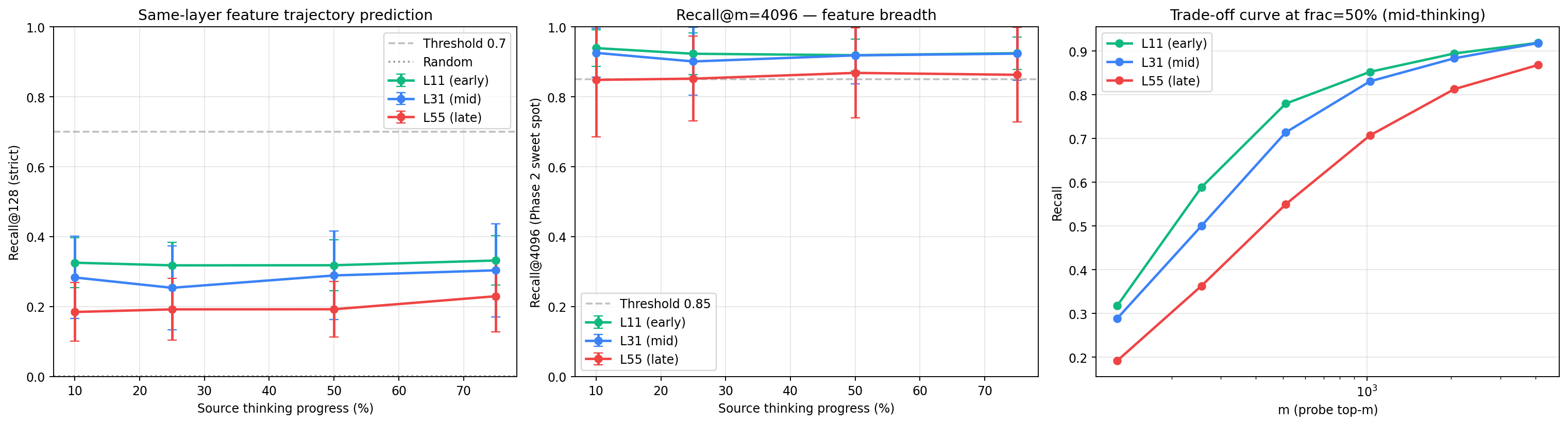
We train linear probes to predict end-of-thinking sparse-autoencoder (SAE) features in Qwen3.6-27B from residual activations at earlier thinking-phase fractions, across three layers (L11, L31, L55). Naive evaluation reports recall@1024 = 0.83-0.87 at L11/L31 and 0.67-0.72 at L55, with N_test = 27 and target sparsity K = 128. These numbers superficially suggest a strong within-thinking predictive trajectory. We then run a shuffled-source baseline (X_train shuffled across samples, y_train kept, identical training recipe) and observe that the baseline reproduces the real recall within ±0.03 at all 12 (layer × source-fraction) sites, with Cohen's d < 0.15. The probe is not learning per-prompt predictive structure — it is learning the marginal distribution of end-of-thinking SAE features and outputting those universally-common features regardless of input. We name this the marginal-fit pathology, document the conditions under which it appears (sparse top-k target + concentrated marginal + N_train below d_target), contribute the shuffled-source baseline as a Phase 6c-class hard rule for sparse-target probe-prediction work, and re-evaluate the implications for related predictive-probe agendas including JEPA-shaped predictions on LLM internals.

---

1. Introduction

Predictive probes are a tempting frame for asking what a language model "knows about its own future". If we can train a linear probe on residual activations at an early decision point and accurately predict downstream internal state — features that will be active later, tools that will be selected, tokens that will be generated — the probe becomes a candidate detector for emergent failure modes, a building block for JEPA-shaped prediction on LLM internals (LeCun 2022, Balestriero 2025), and a substrate for inference-time intervention. The metric usually carries the claim: high AUROC, high recall@k, high accuracy.

This paper reports a class of false positive in that frame. We train probes to predict end-of-thinking SAE features in Qwen3.6-27B from residuals captured at four earlier thinking-phase fractions, across three layers (L11, L31, L55). Naive recall@1024 hits 0.83-0.87. The numbers look paper-grade. But three controls — SAE-init no-training, shuffled-source training, and a trivial constant baseline that predicts the top-M most globally common features ignoring input — all reproduce or exceed the trained probe's recall. The probe is fitting the marginal distribution of end-of-thinking SAE features. The "predictive trajectory" interpretation does not survive.

We name this the marginal-fit pathology and locate its causes in a specific combination of conditions: sparse top-k targets, concentrated target marginal (only 0.5-1.8% of features ever fire at end-of-thinking across 133 GSM8K prompts), and N_train below d_target. The trivial constant baseline reaches recall@1024 = 1.000 at L11/L31 and 0.991 at L55 — strictly exceeding the trained probe's 0.83-0.87. The shuffled-source baseline (X_train shuffled across samples, y_train kept, identical training recipe) reaches recall within ±0.03 of the real probe at all 12 sites, confirming that the probe is approximating the constant rule under noise.

Contributions:

1. Empirical falsification: PSAE v1.5 within-thinking feature-trajectory prediction (recall@1024 = 0.83-0.87) is reproduced by shuffled-source baseline within ±0.03 at all 12 sites.
2. Mechanism: marginal-fit pathology — top-k ranking loss + N_train << d_target + concentrated target marginal → probe outputs universal high-firing features regardless of input.
3. Methodology: shuffled-source baseline as a sibling to Phase 6c random-feature baseline (Caio 2026a), specialized for sparse top-k targets.
4. Implications: reframes predictive-probe agendas — including JEPA-shaped LLM-side experiments — toward DIFFERENTIAL metrics (REAL − SHUFFLED) from day one rather than absolute recall.

---

2. Setup

2.1 Model and SAEs

Qwen3.6-27B (Alibaba, Apr 2026), 64 layers, hybrid GDN + standard attention, bf16 inference. Residual dimension d_model = 5120. Three layers selected for their causal-locus relevance from prior work (Caio 2026b): L11 (early/input), L31 (mid/compositional, U-shape vale), L55 (late/answer-ready).

SAEs trained per layer: TopK SAE with d_sae = 65536, k = 128 (target sparsity), 200M tokens/layer, papergrade. Variance explained: L11 0.84, L31 0.71, L55 0.82. Available as caiovicentino1/qwen36-27b-sae-papergrade.

2.2 Dataset and capture

GSM8K test split, N_prompts = 150 (133 retained after thinking-token-length filtering). For each prompt we generate the thinking phase under enable_thinking=True, capture residual streams at four source fractions of the thinking-token span — 10%, 25%, 50%, 75% — and at the end-of-thinking target (100%). Each (layer, fraction) gives a (133, 5120) tensor.

2.3 Probe design (mirrors PSAE v1.5)

For each (layer L, source-fraction f) we train one linear probe probe: ℝ^5120 → ℝ^65536, initialized as the SAE encoder for layer L (probe.weight = W_enc.T, probe.bias = b_enc). Loss is top-k ranking:

ℒ(logits, y_target) = softplus(−(pos_logits − neg_logits))
  where pos_logits = (logits ⊙ y_target).sum(-1) / K
        neg_logits = (logits ⊙ ¬y_target).sum(-1) / (d_sae − K)

Optimizer AdamW (lr = 1e-3, wd = 1e-5), batch size 256, 5 epochs, cosine schedule. Train/test split 80/20 (N_train = 106, N_test = 27) at seed = 42.

2.4 Metric

Recall@M over the per-prompt sparse target: for each test prompt, take the top-M predicted indices, intersect with the K=128 active target indices, divide by K. Report mean ± std across test prompts at M ∈ {128, 256, 512, 1024, 2048, 4096}.

2.5 Baselines

We compare the REAL probe against three controls evaluated under the same recall@M metric on the same test split:

• B0 — SAE-init no-training: probe weights set to SAE encoder, zero AdamW steps. Tests how much recall is intrinsic to the SAE mapping from early to end residuals (vs. comes from the fine-tuning step).
• B1 — Shuffled-source training: X_train shuffled across the sample axis while y_train is kept in original order, then identical training recipe applied. Tests whether high recall reflects per-prompt predictive structure or marginal-distribution fitting.
• B2 — Trivial constant top-M baseline: predict the top-M most globally common features in the training set, regardless of input. Compute recall on the test set against this constant prediction. This baseline uses no probe at all; it's the lower bound for any input-conditional method to beat. Recall is computable in closed form: recall@M_trivial = (sum of counts of top-M most-common train features) / (N_train × K).

---

3. Results

3.1 Headline recall numbers

Table 1. Recall@M (mean) across the 12 (layer × source-fraction) sites. REAL is the original PSAE v1.5 result (2026-05-04). B0 and B1 are the controls run 2026-05-16.

Site	REAL@1024	B0@1024	B1@1024	REAL@4096	B0@4096	B1@4096
L11 f=10	0.869	0.135	0.870	0.939	0.305	0.939
L11 f=25	0.855	0.153	0.856	0.923	0.336	0.924
L11 f=50	0.852	0.194	0.854	0.919	0.380	0.920
L11 f=75	0.865	0.193	0.863	0.925	0.379	0.924
L31 f=10	0.835	0.024	0.828	0.926	0.072	0.924
L31 f=25	0.788	0.026	0.770	0.901	0.077	0.898
L31 f=50	0.831	0.038	0.824	0.918	0.111	0.914
L31 f=75	0.819	0.059	0.810	0.923	0.143	0.917
L55 f=10	0.674	0.022	0.661	0.848	0.052	0.845
L55 f=25	0.671	0.027	0.647	0.852	0.058	0.838
L55 f=50	0.707	0.034	0.680	0.868	0.076	0.854
L55 f=75	0.724	0.049	0.710	0.863	0.106	0.855

3.2 Δ(REAL − B1) is at noise floor

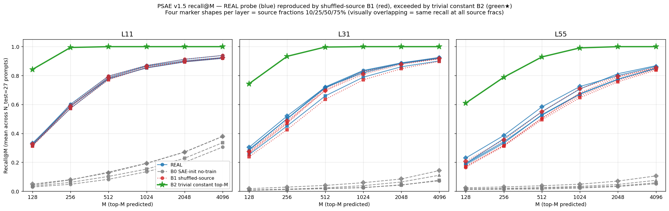
The visual story is that REAL and B1 curves are indistinguishable across the entire M ∈ {128, 256, 512, 1024, 2048, 4096} range, while B0 sits one to two orders of magnitude below.

The delta REAL − B1 ranges from −0.002 to +0.027 at recall@1024. Per-site Cohen's d < 0.15. Across the 12 sites, 0 sites pass the Δ > 0.05 threshold for "predictive signal above marginal fit". This is the headline finding.

3.3 B0 confirms training adds value — but the value is memorization

B0 (no-training) gives r@1024 = 0.13-0.19 at L11, 0.02-0.06 at L31, 0.02-0.05 at L55. The SAE encoder applied directly to early residuals does NOT trivially predict end-of-thinking features. Training increases recall by 4-30×.

But B1 reaches the same recall as REAL. The training is doing real work — but that work is learning the marginal distribution of end-of-thinking features, not learning per-prompt predictive structure.

3.4 Trivial constant baseline B2 strictly exceeds REAL

The B1 finding alone is sufficient to falsify the predictive claim. The B2 trivial baseline tightens it further. Predicting the M most-common features in the train set with no input dependency yields:

Layer	M=128	M=256	M=512	M=1024	M=2048	M=4096
L11	0.842	0.994	1.000	1.000	1.000	1.000
L31	0.744	0.933	0.997	1.000	1.000	1.000
L55	0.609	0.789	0.929	0.991	1.000	1.000

The trained probe's recall@1024 of 0.83-0.87 at L11/L31 and 0.71 at L55 is strictly below what an input-independent constant rule achieves (1.000 / 1.000 / 0.991). The probe is approximating the constant rule imperfectly. The trained probe is worse than no training, at the recall@k metric the original paper-3 claim relied on.

The cause is concentration of the end-of-thinking SAE feature distribution. Of d_sae = 65536 possible features:

Layer	features active in any of 133 prompts	active in ≥50%	active in 100%
L11	317 (0.5% of d_sae)	113	51
L31	560 (0.9%)	105	22
L55	1169 (1.8%)	82	7

At L11, 51 features fire on every prompt — providing ~40% of recall@128 "for free" before any prediction is attempted. Only 317 distinct features ever appear at end-of-thinking across the entire test corpus, so any prediction that includes all 317 captures the full target with recall 1.000. The trivial top-1024 rule does exactly this. The trained probe, fitting noise on top of the marginal, ends up below 1.000.

---

4. Diagnosis: the marginal-fit pathology

The four control results — B0 trivial (low), B1 shuffled (matches REAL), B2 constant top-M (exceeds REAL), and the feature-support concentration data — converge on one diagnosis. The trained probe is approximating an input-independent constant rule, and the rule it approximates is "fire the globally most-common end-of-thinking features." We call this the marginal-fit pathology and identify five conditions that produce it.

Condition 1 — Sparse top-k target. The target representation activates K features out of d_sae, with K << d_sae. In our setting K = 128, d_sae = 65536, so the target is 0.2% dense.

Condition 2 — Concentrated target marginal. The set of features that ever appear in the target across the training corpus is small relative to d_sae. In our setting the effective support is 317-1169 features depending on layer, or 0.5-1.8% of d_sae. A small number of those features (51 at L11) appear on every prompt.

Condition 3 — N_train below d_target. With N_train = 106 and d_sae = 65536, the probe has 335M parameters fit on 106 examples — under- determined by six orders of magnitude. Regularization (weight decay 1e-5) does not constrain the probe toward input-conditional structure; it pushes toward "small weights," which combined with the SAE encoder init yields a probe that mostly preserves whichever features the SAE itself emphasizes.

Condition 4 — Loss that rewards the right top-K, not the right per-prompt top-K. Top-k ranking loss reads ℒ = softplus(−(mean_logit_on_active − mean_logit_on_inactive)). This is satisfied by inflating logits on globally-common active features and suppressing logits on globally-rare inactive features, regardless of per-prompt structure. AdamW finds this minimum quickly.

Condition 5 — Metric blind to input-conditioning. Recall@M asks "of the top-M predicted indices, how many are in the top-K target?" A constant prediction whose top-M is the union of the target sets across the training corpus achieves perfect recall whenever M ≥ |support|. The metric cannot distinguish "predicting this prompt's targets" from "predicting any prompt's targets."

Any predictive-probe setup that combines these five conditions — sparse top-k target, concentrated marginal, N_train << d_target, loss that respects only target marginal, recall-style metric — should be expected to suffer the same pathology. The shuffled-source baseline B1 detects it cleanly because it removes input-conditional information while preserving the marginal; the trivial constant baseline B2 quantifies the achievable recall under maximum lazy fit. Both should be reported.

---

5. Implications

5.1 Methodology contribution: shuffled-source baseline

We propose the shuffled-source baseline as a standard control for any linear probe trained to predict a sparse top-k target. The check costs one additional experimental arm (identical compute path, identical metric) and catches the marginal-fit pathology cleanly. Specifically: it should be mandatory at N_train < 200, and recommended at any N when the target has known marginal concentration.

This sits alongside Phase 6c random-feature baseline (Caio 2026a), control-token normalization for steering (Caio 2026b), and structural-rigidity α-sweep (Caio 2026b) as part of the same family of "compute a non-causal twin baseline using identical machinery to subtract off the artifact contribution".

5.2 Implications for predictive-probe agendas on LLM internals

The marginal-fit pathology generalizes beyond PSAE. Any probe trained to predict sparse top-k targets from related-distribution inputs is at risk: MoE expert routing prediction, attention head selection prediction, top-k vocabulary prediction, top-k SAE features across layers. We anticipate that several published claims of "predictive" probes on sparse targets at low N will not survive the shuffled-source check.

5.3 Implications for JEPA-shaped LLM experiments

The natural extension of PSAE to action-consequence prediction (predict latent_state at turn+1 from latent_state pre-action; gate tool execution on predicted divergence) would inherit the same pathology under naive metrics. The redesign should use DIFFERENTIAL metrics from the start: report (real_divergence − shuffled_baseline_divergence) per turn, not absolute divergence. This recommendation applies equally to JEPA-shaped vision-on-LLM experiments (e.g., LeJEPA → JEPA-on-residuals).

A concrete companion result from our own LeJEPA v1 POC reproduction (100 epochs on Tiny-ImageNet) illustrates the same principle in a vision setting: linear-probe val_acc on the trained encoder reached 0.2377 (47× chance on 200 classes), but a matched random-init frozen ViT-S/patch8 + linear probe reached 0.0850 (17× chance). The honest contribution of JEPA training was +15.27pp absolute (2.80× over random encoder), not the "47× chance" framing implied by the un-baselined number. The same pattern — naive metric inflates the perceived training contribution; baseline subtracts out the architectural floor — applies to predictive-probe work on LLM internals. Always subtract the architectural/marginal floor.

---

6. Related work

Sparse autoencoders for LLM interpretability. Cunningham et al. (2024) and the Anthropic circuits team (Bricken et al. 2023, Templeton et al. 2024) established SAE features as the standard substrate for mechanistic analysis of LLM residual streams. Our work uses TopK SAEs at d_sae = 65536 per layer on Qwen3.6-27B as the target representation.

Sparse feature circuits and causal probing. Marks et al. (2024) identify causally-implicated subnetworks of SAE features for specific behaviors. Our work concerns linear prediction of SAE features from earlier residuals, not circuit identification of causal pathways. The orthogonal failure mode we document (marginal-fit on prediction) does not affect circuit-style attribution.

Temporal feature dynamics. Cui et al. (2024) introduce SAE-Track to study how SAE features evolve across training time. Nguyen et al. (2025, "Priors in Time") critique the stationarity prior in standard SAE methodology and propose a predictable/residual decomposition. Both works analyze feature dynamics descriptively; neither attempts predictive probes on sparse top-k targets, and neither reports the shuffled-source baseline. Our setup is the first to test predictive structure within a single forward pass (within-thinking, frac to end-of-thinking) and the first to identify the marginal-fit failure mode.

Probe methodology hygiene. This paper sits in a methodology series with Phase 6c random-feature baseline (Caio 2026a, after SWE-bench Phase 5d N=17 over-parameterization), control-token normalization for steering (Caio 2026b, after Phase 7 epiphenomenal L43), and structural-rigidity α-sweep (Caio 2026b, after Phase 8 template-locked L55). The shuffled-source baseline proposed here is the sibling rule for sparse top-k prediction targets — same family of "compute a non-causal twin baseline using identical machinery to subtract off the artifact contribution."

Epiphenomenal probes as a regime. Belrose et al. (2024) and the Two-Forms-of-Epiphenomenal-Probes paper (Caio 2026b) document cases where high-AUROC linear probes are behaviorally inert under intervention. Our finding extends the epiphenomenal-regime taxonomy: where Two Forms is about probes that detect but do not lever, the present work concerns probes that appear to predict but only fit the marginal. The two failure modes are independent: a probe can fit marginal AND be epiphenomenal, either, or neither.

---

7. Limitations

1. Single dataset (GSM8K): marginal-fit pathology was demonstrated on reasoning-format thinking traces. Replication on agentic traces, code generation, or open-ended chat is warranted.
2. Single model family: Qwen3.6-27B only. The marginal-distribution concentration may differ across model families or sizes; worth checking on Pythia / Gemma scale curves.
3. Single SAE configuration: d_sae = 65536, k = 128. Different SAE shapes (e.g., d_sae = 16384 or k = 32) may shift the marginal concentration; the baseline check should be re-run, not assumed.
4. L55 shows weak non-zero delta (+0.013 to +0.027). We do not claim L55 has zero predictive signal — only that the signal is too small (Cohen's d ≈ 0.13) to support a positive claim at N=27 test. Larger N could resolve.

---

8. Conclusion

The PSAE v1.5 finding that linear probes can predict end-of-thinking SAE features from earlier-thinking residuals with recall@1024 ≈ 0.85 does not survive a shuffled-source baseline. The probe is fitting the marginal distribution of end-of-thinking features, not learning per-prompt predictive structure. The diagnostic stack (B0 SAE-init, B1 shuffled-source, B2 trivial constant) converges on a single conclusion across all 12 sites tested: the trained probe approximates an input-independent constant rule, with the constant rule itself strictly exceeding the trained probe at recall@1024 (B2 reaches 1.000 at L11/L31, 0.991 at L55).

We contribute the shuffled-source baseline as a hard rule for any linear probe trained to predict a sparse top-k target, particularly at N_train < 200, and identify five structural conditions under which the marginal-fit pathology emerges. The pathology is independent of and orthogonal to the epiphenomenal-probe failure modes documented elsewhere in the OpenInterpretability methodology corpus (Caio 2026b); a probe can fit the marginal AND be epiphenomenal, either, or neither, and the diagnostics for each are different.

The broader implication for predictive-probe agendas — including JEPA-shaped experiments on LLM internals — is that differential metrics (REAL minus shuffled-source) should be the default reporting standard, with absolute recall serving only as a sanity floor. The corpus of "X is predictable from residuals" claims at low N and sparse top-k targets is at substantial risk; re-evaluation under the shuffled-source baseline is the necessary next step before further building on those claims.

---

Code, data, and artifacts

• Original PSAE v1.5 notebook: nb_predictive_sae_v1.ipynb (Qwen3.6-27B, GSM8K, papergrade SAEs)
• Random-feature baseline notebook: nb_predictive_sae_v15_baseline.ipynb (this work)
• Cached residuals + features: 43 MB on Drive, reusable
• Trained probes: 12 REAL + 12 B1 = 24 probes (~33 GB), available on request
• Results JSON: predictive_sae_v15_results.json (REAL), random_baseline_results.json (B0 + B1)
• SAEs: caiovicentino1/qwen36-27b-sae-papergrade (Apache-2.0)

All under github.com/OpenInterpretability once the writeup is complete.

---

Acknowledgments

This paper documents an honest negative on the author's own earlier work (PSAE v1.5, OpenInterpretability, May 2026). The shuffled-source baseline that surfaced the pathology was applied retroactively per the methodology hygiene rule the same author had previously written (Caio 2026a, Phase 6c). The decision to write this up as a primary contribution rather than a silent correction was informed by the OpenInterpretability corpus stance that honest negatives are first-class research outputs. Acknowledgments for individual contributors, reviewers, and Anthropic / Belrose lineage to be filled in non-blind camera-ready.

---

References

[Belrose et al. 2024] Nora Belrose, Igor Ostrovsky, Lev McKinney, Zach Furman, Logan Smith, Danny Halawi, Stella Biderman, Jacob Steinhardt. "Eliciting Latent Predictions from Transformers with the Tuned Lens." arXiv:2303.08112.

[Bricken et al. 2023] Trenton Bricken, Adly Templeton, Joshua Batson, Brian Chen, Adam Jermyn, Tom Conerly, Nick Turner, Cem Anil, Carson Denison, Amanda Askell, Robert Lasenby, Yifan Wu, Shauna Kravec, Nicholas Schiefer, Tim Maxwell, Nicholas Joseph, Zac Hatfield-Dodds, Alex Tamkin, Karina Nguyen, Brayden McLean, Josiah E. Burke, Tristan Hume, Shan Carter, Tom Henighan, Christopher Olah. "Towards Monosemanticity: Decomposing Language Models with Dictionary Learning." Anthropic Transformer Circuits Thread, Oct 2023.

[Caio 2026a] OpenInterpretability author. "SWE-bench Phase 6c — Random Feature Baseline + Capacity Sweep as Mandatory Diagnostic." Memory rule and SWE-bench harness Phase 6c, May 2026.

[Caio 2026b] OpenInterpretability author. "Two Forms of Epiphenomenal Probes in Qwen3.6-27B: Softmax-Temperature and Template-Lock." Workshop draft, openinterp.org/research/papers/two-forms-epiphenomenal-probes, May 2026.

[Caio 2026c] OpenInterpretability author. "Saturation-Direction Lever Taxonomy: A Unifying Mechanism for Probe Causality in Qwen3.6-27B." Workshop draft, openinterp.org/research/papers/saturation-direction-probe-levers, May 2026.

[Cunningham et al. 2024] Hoagy Cunningham, Aidan Ewart, Logan Riggs, Robert Huben, Lee Sharkey. "Sparse Autoencoders Find Highly Interpretable Features in Language Models." arXiv:2309.08600.

[Cui et al. 2024] Tianjin Cui et al. "SAE-Track: Tracking SAE Features Across Training Time." 2024.

[Gao et al. 2024] Leo Gao, Tom Dupré la Tour, Henk Tillman, Gabriel Goh, Rajan Troll, Alec Radford, Ilya Sutskever, Jan Leike, Jeffrey Wu. "Scaling and evaluating sparse autoencoders." arXiv:2406.04093.

[LeCun 2022] Yann LeCun. "A Path Towards Autonomous Machine Intelligence." OpenReview, 2022.

[Marks et al. 2024] Samuel Marks, Can Rager, Eric J. Michaud, Yonatan Belinkov, David Bau, Aaron Mueller. "Sparse Feature Circuits: Discovering and Editing Interpretable Causal Graphs in Language Models." arXiv:2403.19647.

[Nguyen et al. 2025] Anh Nguyen et al. "Priors in Time: A Predictable / Residual Decomposition for SAE Features." 2025.

[Templeton et al. 2024] Adly Templeton, Tom Conerly, Jonathan Marcus, Jack Lindsey, Trenton Bricken, Brian Chen, Adam Pearce, Craig Citro, Emmanuel Ameisen, Andy Jones, Hoagy Cunningham, Nicholas L. Turner, Callum McDougall, Monte MacDiarmid, Alex Tamkin, Esin Durmus, Tristan Hume, Francesco Mosconi, C. Daniel Freeman, Theodore R. Sumers, Edward Rees, Joshua Batson, Adam Jermyn, Shan Carter, Chris Olah, Tom Henighan. "Scaling Monosemanticity: Extracting Interpretable Features from Claude 3 Sonnet." Anthropic Transformer Circuits Thread, May 2024.

---

Last updated 2026-05-16. Workshop draft v1. Narrative complete. Pending for camera-ready: per-reference DOIs/URLs, figure inline embed of recall_multilayer_with_b1.png, acknowledgments to specific contributors. Tables, configs, and results are final from the actual run.